
Hands-on tutorial
Here we give some examples of generally-used steps to obtain fluxes, spectra and Ogives. This is just the commonly done procedures, but more steps and procedures can be done (and sometimes should, depending on the data).
Quality control procedures
Here we give a brief example of how to perform some simple quality control procedures using Pymicra, which is generally the first thing to be done with a new dataset on our hands. We will use some 1-hour files as examples for this procedure. The following lines simply load the necessary packages.
In [1]: import pymicra as pm

In [2]: pm.notation = pm.Notation()

In [3]: import pandas as pd

In [4]: pd.options.display.max_rows = 30 # This line just alters the visualization
The first thing is to read the files so as to have a list of file paths. We will need a configuration file since we must know what is in each column to be able to perform the quality control correctly.
In [5]: import pymicra as pm

In [6]: from glob import glob

In [7]: fconfig = pm.fileConfig('../examples/lake.config')

In [8]: fnames = glob('../examples/ex_data/***.csv')

In [9]: fnames
Out[9]:
['../examples/ex_data/20131108-1200.csv',
 '../examples/ex_data/20131108-1600.csv',
 '../examples/ex_data/20131108-1300.csv',
 '../examples/ex_data/20131108-1900.csv',
 '../examples/ex_data/20131108-1700.csv',
 '../examples/ex_data/20131108-1800.csv',
 '../examples/ex_data/20131108-1000.csv']
There are two functions that currently do the quality control in Pymicra: pm.util.qc_replace() and pm.util.qc_discard(). They are separated only for simplicity, but are meant to be used in sequence (first qc_replace() and then qc_discard()).
The first one, pm.util.qc_replace(), is intended for quality control procedures that can “fix” certain data by removing or interpolating a few “bad points”. At this time it checks for file dates and file lines and it filters the data for spikes, NaNs and out-of-bounds values. Every time one of those latter one is found they are interpolated with either the linear trend of the dataset or a simple linear interpolation. If at the end the number of interpolations is higher than a user-defined threshold than the run fails the quality control and is discarded. Thus we can do the first part of the quality control with
In [10]: pm.util.qc_replace(fnames, fconfig,
   ....:     file_lines=72000,
   ....:     nans_test=True,
   ....:     lower_limits=dict(theta_v=10, mrho_h2o=0, mrho_co2=0),
   ....:     upper_limits=dict(theta_v=45),
   ....:     spikes_test=True,
   ....:     spikes_func=lambda x: (abs(x - x.median()) > (5./0.6745)*x.mad()),
   ....:     visualize_spikes=False,
   ....:     chunk_size=2400,
   ....:     max_replacement_count=1440,
   ....:     outdir='../examples/passed_1st',
   ....:     replaced_report='../examples/rrep.txt')
   ....:
20131108-1200.csv
Passed all tests
Re-writing ../examples/ex_data/20131108-1200.csv

20131108-1600.csv
Passed all tests
Re-writing ../examples/ex_data/20131108-1600.csv

20131108-1300.csv
Passed all tests
Re-writing ../examples/ex_data/20131108-1300.csv

20131108-1900.csv
Passed all tests
Re-writing ../examples/ex_data/20131108-1900.csv

20131108-1700.csv
Passed all tests
Re-writing ../examples/ex_data/20131108-1700.csv

20131108-1800.csv
Passed all tests
Re-writing ../examples/ex_data/20131108-1800.csv

20131108-1000.csv
Passed all tests
Re-writing ../examples/ex_data/20131108-1000.csv

                           control  percent
total                            7    100.0
failed lines test                0      0.0
failed replacement test          0      0.0
passed all tests                 7    100.0
Runs with replaced nans          0      0.0
Runs with replaced bound         0      0.0
Runs with replaced spikes        7    100.0
Out[10]:
    passed all tests              total  failed lines test  Runs with replaced nans  \
0  20131108-1200.csv  20131108-1200.csv                NaN                      0.0
1  20131108-1600.csv  20131108-1600.csv                NaN                      0.0
2  20131108-1300.csv  20131108-1300.csv                NaN                      0.0
3  20131108-1900.csv  20131108-1900.csv                NaN                      0.0
4  20131108-1700.csv  20131108-1700.csv                NaN                      0.0
5  20131108-1800.csv  20131108-1800.csv                NaN                      0.0
6  20131108-1000.csv  20131108-1000.csv                NaN                      0.0

   Runs with replaced bound  Runs with replaced spikes  failed replacement test
0                       0.0                       99.0                      NaN
1                       0.0                       42.0                      NaN
2                       0.0                      112.0                      NaN
3                       0.0                       57.0                      NaN
4                       0.0                       47.0                      NaN
5                       0.0                       68.0                      NaN
6                       0.0                      194.0                      NaN
This command effectively does the first part of the quality control. There are other options that aren’t used here but let’s go through the options we used
- file_lines tells the function the amount of lines you expect the files to have. Anything different from that
number means that there was a problem while collecting the data and that file is discarded
- nans_test=True means you want to check for “Not a Number”s, or missing numbers. If one is found it is
interpolated
- lower_limits and upper_limits provide the bounds for the data. Any data
that falls outside these bounds is interpolated. Usually it is suggested that at least the concentrations have 0 as lower limits. In the previous example we considered that virtual temperatures lower than 10 C or higher than 45 C, given the site atmospheric conditions.
- spikes_test tells the function whether to test for spikes or not. Spikes are interpolated over.
- spikes_func every point is tested for spikes using this function. If the result if True, it
is considered a spike. Any Pandas function works here, as x in this case is a pandas DataFrame.
- visualize_spikes decides if you want to see the points you are considering as spikes or not. A matplotlib
plot appears on screen. This is good for the first iterations of the quality control, so you can calibrate your spike parameters and see if your spikes test is really doing what you think it’s doing.
- max_replacement_count sets the maximum number of replaces values a run can have before it is discarded.
This included replacements from the NaNs test, bounds test and spikes test.
- outdir is the path to the directory where the quality-controlled files will be copied.
- replaced_report is the path to a file that will be created with a detailed report on the replacements that were made.
Note
More options are available for the function. Please read the documentation for pymicra.util.qc_replace() for details.
With this function, all the runs that passed our quality control were fixed for the spikes and NaNs that were found and were copied to outdir. The second step is to get these files and apply the second part of the quality control procedure, pymicra.util.qc_discard(). This second part applies tests that, if turn out to fail, there is no way to recover the data and the dataset is simply discarded. The tests are the Standard Deviation (STD) test and the Maximum difference (or stationarity) test.
The STD test separates the run into chunks (of length given by chunk_size) and takes the STD of each chunk. If it is smaller than a certain threshold, than the run is discarded. The Max. diff. test can test for different things, depending on the parameters. The most common use perhaps is to use the maxdif_trend keyword to get the low-frequency variations (low-frequency trend) by doing a moving median and taking out the absolute difference between the higher and the lower values of this trend. If it is higher than a certain value the run is considered non-stationary and discarded. It is kept otherwise. There are more options and more things to do, so be sure to read the docs for pymicra.util.qc_discard().
Below is an example of a simple quality-control procedure done using the data that passed the previous procedure.
In [11]: fnames = sorted(glob('../examples/passed_1st/***.csv'))

In [12]: fnames
Out[12]:
['../examples/passed_1st/20131108-1000.csv',
 '../examples/passed_1st/20131108-1200.csv',
 '../examples/passed_1st/20131108-1300.csv',
 '../examples/passed_1st/20131108-1600.csv',
 '../examples/passed_1st/20131108-1700.csv',
 '../examples/passed_1st/20131108-1800.csv',
 '../examples/passed_1st/20131108-1900.csv']

In [13]: pm.util.qc_discard(fnames, fconfig,
   ....: std_limits = dict(u=0.03, v=0.03, w=0.01, theta_v=0.02),
   ....: std_detrend=dict(how='linear'),
   ....: chunk_size=1200,
   ....: dif_limits = dict(u=5.0, v=5.0, theta_v=2.0),
   ....: maxdif_trend=dict(how='movingmedian', window= 600),
   ....: failverbose=True,
   ....: failshow=True,
   ....: outdir='../examples/passed_2nd',
   ....: summary_file='2nd_filter_summary.csv',
   ....: full_report='2nd_full_report.csv')
   ....:
20131108-1000.csv
20131108-1000.csv : !FAILED failed maxdif test test!

Failed variable(s): u

20131108-1200.csv
20131108-1200.csv : !FAILED failed maxdif test test!

Failed variable(s): v

20131108-1300.csv
Passed all tests
Re-writing ../examples/passed_1st/20131108-1300.csv

20131108-1600.csv
Passed all tests
Re-writing ../examples/passed_1st/20131108-1600.csv

20131108-1700.csv
Passed all tests
Re-writing ../examples/passed_1st/20131108-1700.csv

20131108-1800.csv
Passed all tests
Re-writing ../examples/passed_1st/20131108-1800.csv

20131108-1900.csv
Passed all tests
Re-writing ../examples/passed_1st/20131108-1900.csv

                    control     percent
total                     7  100.000000
failed STD test           0    0.000000
failed maxdif test        2   28.571429
passed all tests          5   71.428571
Out[13]:
    passed all tests              total  failed STD test failed maxdif test
0                NaN  20131108-1000.csv              NaN  20131108-1000.csv
1                NaN  20131108-1200.csv              NaN  20131108-1200.csv
2  20131108-1300.csv  20131108-1300.csv              NaN                NaN
3  20131108-1600.csv  20131108-1600.csv              NaN                NaN
4  20131108-1700.csv  20131108-1700.csv              NaN                NaN
5  20131108-1800.csv  20131108-1800.csv              NaN                NaN
6  20131108-1900.csv  20131108-1900.csv              NaN                NaN
After the previous example you should be left with reasonably quality-controlled dataset. We used the following options in this case:
- std_limits gives the minimum value for the STD before it is considered too small and the run is discarded. So,
values of STD larger than std_limits are fine.
- std_detrend gives the detrending options to use before taking the STD in the STD test.
- chunk_size size of chunks in which to separate the data for the STD test.
- dif_limits are the maximum difference between the largest and lowest value in the Max dif (stationarity) test. If the
difference is larger the run is discarded.
- maxdif_trend is the trend to consider when taking the difference between the lowest and highest value.
- failverbose shows extra info on runs that fail any test (like which variable(s) failed).
- failshow plots runs that failed some test on the screen for checking purposes.
As usual, there are more options to this, but this is a basic introduction. With the dataset already corrected and filtered we move on to the processing of data.
Calculating auxiliary variables and units
After reading the data it’s easy to rotate the coordinates. Currently, only the
2D rotation is implemented. But in the future more will come (you can
contribute with another one yourself!). To rotate, use the pm.rotateCoor
function:
In [1]: import pymicra as pm

In [2]: fname = '../examples/ex_data/20131108-1000.csv'

In [3]: fconfig = pm.fileConfig('../examples/lake.config')

In [4]: data, units = pm.timeSeries(fname, fconfig, parse_dates=True)

In [5]: data = data.rotateCoor(how='2d')

In [6]: print(data.with_units(units).mean())
u         <meter / second>            6.021737e+00
v         <meter / second>            2.271683e-14
w         <meter / second>            1.178001e-16
theta_v   <degC>                      2.764434e+01
mrho_h2o  <millimole / meter ** 3>    1.169865e+03
mrho_co2  <millimole / meter ** 3>    1.466232e+01
p         <kilopascal>                9.913677e+01
theta     <degC>                      3.127128e+01
dtype: float64
As you can see, the u, v, w components have been rotated and v and w
mean are zero.
Pymicra has a very useful function called preProcess which “expands” the
variables in the dataset by using the original variables to calculate new ones,
such as mixing ratios, moist and dry air densities etc. In the process some
units are also converted, such as temperature units, which are converted to
Kelvin, if they are in Celsius. The preProcess function has some options to
calculate some variables in determined ways and is very “verbose”, so as to
show the user exactly what it is doing:
In [7]: data = pm.micro.preProcess(data, units, expand_temperature=True,
   ...:     use_means=False, rho_air_from_theta_v=True, solutes=['co2'])
   ...:
Beginning of pre-processing ...
Rotating data with 2d method ... Done!
Converting theta_v and theta to kelvin ... Done!
Sonic temperature not found ... trying to calculate it ... not possible with current variables!
Didn't locate mass density of h2o. Trying to calculate it ... Done!
Moist air density not present in dataset
Calculating rho_air = p/(Rdry * theta_v) ... Done!
Calculating dry_air mass_density = rho_air - rho_h2o ... Done!
Dry air molar density not in dataset
Calculating dry_air molar_density = rho_dry / dry_air_molar_mass ... Done!
Calculating specific humidity = rho_h2o / rho_air ... Done!
Calculating h2o mass mixing ratio = rho_h2o / rho_dry ... Done!
Calculating h2o molar mixing ratio = rho_h2o / rho_dry ... Done!
Didn't locate mass density of co2. Trying to calculate it ... Done!
Calculating co2 mass concentration (g/g) = rho_co2 / rho_air ... Done!
Calculating co2 mass mixing ratio = rho_co2 / rho_dry ... Done!
Calculating co2 molar mixing ratio = mrho_co2 / mrho_dry ... Done!
Pre-processing complete.


In [8]: print(data.with_units(units).mean())
u         <meter / second>            6.021737e+00
v         <meter / second>           -9.655764e-16
w         <meter / second>            2.983030e-17
theta_v   <kelvin>                    3.007943e+02
mrho_h2o  <millimole / meter ** 3>    1.169865e+03
mrho_co2  <millimole / meter ** 3>    1.466232e+01
p         <kilopascal>                9.913677e+01
theta     <kelvin>                    3.044213e+02
rho_h2o   <kilogram / meter ** 3>     2.107547e-02
rho_air   <kilogram / meter ** 3>     1.148149e+00
rho_dry   <kilogram / meter ** 3>     1.127073e+00
mrho_dry  <mole / meter ** 3>         3.891223e+01
q         <dimensionless>             1.835686e-02
r_h2o     <dimensionless>             1.870102e-02
mr_h2o    <dimensionless>             3.006698e-02
rho_co2   <kilogram / meter ** 3>     6.452812e-04
conc_co2  <dimensionless>             5.620179e-04
r_co2     <dimensionless>             5.725280e-04
mr_co2    <dimensionless>             3.768047e-04
dtype: float64
Note that our dataset now has many other variables and that the temperatures are now in Kelvin. Note also that you must, at this point, specify which solutes you wish to consider. The only solute that Pymicra looks for by default is water vapor.
It is recommended that you carefully observe the output of preProcess to
see if it’s doing what you think it’s doing and to analyse its calculation
logic. By doing that you can have a better idea of what it does without having
to check the code, and how to prevent it from doing some calculations you don’t
want. For example, if you’re not happy with the way it calculates moist air
density, you can calculate it yourself by extracting Numpy_ arrays using the
.values method:
T = data['theta'].values
P = data['p'].values
water_density = data['mrho_h2o'].values
data['rho_air'] = my_rho_air_calculation(T, P, water_density)
Next we calculate the fluctuations. The way to do that is with the detrend()
function/method.
In [9]: ddata = data.detrend(how='linear', units=units, ignore=['p', 'theta'])

In [10]: print(ddata.with_units(units).mean())
u'         <meter / second>            8.377498e-09
v'         <meter / second>            8.453924e-09
w'         <meter / second>            1.020185e-10
theta_v'   <kelvin>                    6.261396e-09
mrho_h2o'  <millimole / meter ** 3>    1.206199e-07
mrho_co2'  <millimole / meter ** 3>   -5.600283e-10
rho_h2o'   <kilogram / meter ** 3>     7.408674e-13
rho_air'   <kilogram / meter ** 3>     3.606646e-12
rho_dry'   <kilogram / meter ** 3>     9.526920e-12
mrho_dry'  <mole / meter ** 3>        -2.731307e-09
q'         <dimensionless>             2.835312e-13
r_h2o'     <dimensionless>             2.301367e-12
mr_h2o'    <dimensionless>             1.006615e-11
rho_co2'   <kilogram / meter ** 3>     2.048293e-14
conc_co2'  <dimensionless>            -1.126744e-14
r_co2'     <dimensionless>            -4.827255e-15
mr_co2'    <dimensionless>            -1.057082e-14
dtype: float64
Note the ignore keyword with which you can pass which variables you don’t
want fluctuations of. In our case both the pressure fluctuations and the
thermodynamic temperature (measured with the LI7500 and the datalogger’s
internal thermometer) can’t be properly measured with the sensors used. Passing
these variables as ignored will prevent Pymicra from calculating these
fluctuations, which later on prevents it from inadvertently using the
fluctuations of these variables with these sensors when calculating fluxes.
theta fluctuations will instead be calculated with virtual temperature
fluctuations and pressure fluctuations are generally not used.
The how keyword supports 'linear', 'movingmean',
'movingmedian', 'block' and 'poly'. Each of those (with the
exception of 'block' and 'linear') are passed to Pandas or Numpy
(pandas.rolling_mean, pandas.rolling_median and numpy.polyfit) and
support their respective keywords, such as data.detrend(how='movingmedian',
units=units, ignore=['theta', 'p']), min_periods=1) to determine the minimum
number of observations in window required to have a value.
Now we must expand our dataset with the fluctuations by joining DataFrames:
In [11]: data = data.join(ddata)

In [12]: print(data.with_units(units).mean())
u          <meter / second>            6.021737e+00
v          <meter / second>           -9.655764e-16
w          <meter / second>            2.983030e-17
theta_v    <kelvin>                    3.007943e+02
mrho_h2o   <millimole / meter ** 3>    1.169865e+03
mrho_co2   <millimole / meter ** 3>    1.466232e+01
p          <kilopascal>                9.913677e+01
theta      <kelvin>                    3.044213e+02
rho_h2o    <kilogram / meter ** 3>     2.107547e-02
rho_air    <kilogram / meter ** 3>     1.148149e+00
rho_dry    <kilogram / meter ** 3>     1.127073e+00
mrho_dry   <mole / meter ** 3>         3.891223e+01
q          <dimensionless>             1.835686e-02
r_h2o      <dimensionless>             1.870102e-02
mr_h2o     <dimensionless>             3.006698e-02
                                           ...
w'         <meter / second>            1.020185e-10
theta_v'   <kelvin>                    6.261396e-09
mrho_h2o'  <millimole / meter ** 3>    1.206199e-07
mrho_co2'  <millimole / meter ** 3>   -5.600283e-10
rho_h2o'   <kilogram / meter ** 3>     7.408674e-13
rho_air'   <kilogram / meter ** 3>     3.606646e-12
rho_dry'   <kilogram / meter ** 3>     9.526920e-12
mrho_dry'  <mole / meter ** 3>        -2.731307e-09
q'         <dimensionless>             2.835312e-13
r_h2o'     <dimensionless>             2.301367e-12
mr_h2o'    <dimensionless>             1.006615e-11
rho_co2'   <kilogram / meter ** 3>     2.048293e-14
conc_co2'  <dimensionless>            -1.126744e-14
r_co2'     <dimensionless>            -4.827255e-15
mr_co2'    <dimensionless>            -1.057082e-14
Length: 36, dtype: float64
Creating a site configuration file
In order to use some micrometeorological function, we need a site configuration
object, or site object. This object tells Pymicra how the instruments are organized
and how is experimental site (vegetation, roughness length etc.). This object is created
with the siteConfig() call and the easiest way is to use it with a site config file. This
is like a fileConfig file, but simpler and for the micrometeorological aspects of the site.
Consider this example of a site config file, saved at ../examples/lake.site:
description         = "Site configurations for the lake island"

measurement_height  = 2.75  # m
canopy_height       = 0.1   # m
displacement_height = 0.05  # m
roughness_length    = .01   # m
As in the case of fileConfig, the description is optional, but is handy for
organization purposes and printing on screen.
The measurement_height keyword is the general measurement height to be used
in the calculation, generally taken as the sonic anemometer height (in meters).
The canopy_height keyword is what it sounds like. Should be the mean canopy
height in meters. The displacement_height is the zero-plane displacement
height. If it is not given, it’ll be calculated as 2/3 of the mean canopy
height.
The roughness_length is the roughness length in meters.
The creation of the site config object is done as
In [13]: siteconf = pm.siteConfig('../examples/lake.site')

In [14]: print(siteconf)
<pymicra.siteConfig> object
Site configurations for the lake island
----
altitude               None
canopy_height           0.1
displacement_height    0.05
from_file              None
instruments_height     None
latitude               None
longitude              None
measurement_height     2.75
roughness_length       0.01
dtype: object
Extracting fluxes
Finally, we are able to calculate the fluxes and turbulent scales. For that we
use the eddyCovariance function along with the get_turbulent_scales
keyword (which is true by default). Again, it is recommended that you carefully
check the output of this function before moving on:
In [15]: results = pm.micro.eddyCovariance(data, units, site_config=siteconf,
   ....:     get_turbulent_scales=True, wpl=True, solutes=['co2'])
   ....:
Beginning Eddy Covariance method...
Fluctuations of theta not found. Will try to calculate it with theta' = (theta_v' - 0.61 theta_mean q')/(1 + 0.61 q_mean ... done!
Calculating fluxes from covariances ... done!
Applying WPL correction for water vapor flux ... done!
Applying WPL correction for latent heat flux using result for water vapor flux ... done!
Re-calculating cov(mrho_h2o', w') according to WPL correction ... done!
Applying WPL correction for F_co2 ... done!
Re-calculating cov(mrho_co2', w') according to WPL correction ... done!
Beginning to extract turbulent scales...
Data seems to be covariances. Will it use as covariances ...
Calculating the turbulent scales of wind, temperature and humidity ... done!
Calculating the turbulent scale of co2 ... done!
Calculating Obukhov length and stability parameter ... done!
Calculating turbulent scales of mass concentration ... done!
Done with Eddy Covariance.


In [16]: print(results.with_units(units).mean())
tau            <kilogram / meter / second ** 2>     1.957307e-01
H              <watt / meter ** 2>                  5.083720e+01
Hv             <watt / meter ** 2>                  7.453761e+01
E              <millimole / meter ** 2 / second>    7.007486e+00
LE             <watt / meter ** 2>                  3.063926e+02
F_co2          <millimole / meter ** 2 / second>    2.648931e-04
u_star         <meter / second>                     4.128863e-01
theta_v_star   <kelvin>                             1.566857e-01
theta_star     <kelvin>                             1.068650e-01
mrho_h2o_star  <millimole / meter ** 3>             1.697195e+01
mrho_co2_star  <millimole / meter ** 3>             6.415643e-04
Lo             <meter>                             -8.342964e+01
zeta           <dimensionless>                     -3.236260e-02
q_star         <dimensionless>                      2.663024e-04
conc_co2_star  <dimensionless>                      2.459169e-08
dtype: float64
Note that once more we must list the solutes available.
Note also that the units dictionary is automatically updated at with every
function and method with the new variables created and their units! That way if
you’re in doubt of which unit the outputs are coming, just check units
directly or with the .with_units() method.
Check out the example to get fluxes of many files here and download the example data here.
The output of this file is
                                                 tau                   H                  Hv                                 E                  LE  \
                    <kilogram / meter / second ** 2> <watt / meter ** 2> <watt / meter ** 2> <millimole / meter ** 2 / second> <watt / meter ** 2>
2013-11-08 10:00:00                         0.195731           50.837195           74.537609                          7.007486          306.392623
2013-11-08 12:00:00                         0.070182           -7.116972           14.737946                          6.647450          290.331014
2013-11-08 13:00:00                         0.059115           -3.325774           12.743194                          4.875838          212.906974
2013-11-08 16:00:00                         0.017075          -13.847040           -4.131275                          2.961474          128.982980
2013-11-08 17:00:00                         0.003284           -5.557620           -2.525949                          0.931213           40.576805
2013-11-08 18:00:00                         0.026564           -6.632330           -2.782190                          1.184226           51.654208
2013-11-08 19:00:00                         0.044550          -14.860873          -11.991508                          0.925637           40.476446

                              u_star theta_v_star theta_star            mrho_h2o_star          Lo            zeta          q_star
                    <meter / second>     <kelvin>   <kelvin> <millimole / meter ** 3>     <meter> <dimensionless> <dimensionless>
2013-11-08 10:00:00         0.412886     0.156686   0.106865                16.971952  -83.429641       -0.032363        0.000266
2013-11-08 12:00:00         0.247697     0.051834  -0.025031                26.837060  -90.992476       -0.029673        0.000423
2013-11-08 13:00:00         0.227652     0.048903  -0.012763                21.417958  -81.621514       -0.033080        0.000338
2013-11-08 16:00:00         0.122980    -0.029651  -0.099383                24.080946   39.583979        0.068209        0.000384
2013-11-08 17:00:00         0.053951    -0.041353  -0.090986                17.260443    5.463569        0.494182        0.000276
2013-11-08 18:00:00         0.153328    -0.016003  -0.038149                 7.723494  113.854892        0.023714        0.000123
2013-11-08 19:00:00         0.198083    -0.053132  -0.065846                 4.672974   56.961515        0.047400        0.000074
Note that the date parsing when reading the file comes is handy now, although
there are computationally faster ways to do it other than setting
parse_dates=True in the timeSeries() call.
Obtaining the spectra
Using Numpy’s fast Fourier transform implementation, Pymicra is also able to extract spectra, co-spectra and quadratures.
We begin normally with out data:
In [17]: import pymicra as pm

In [18]: fname = '../examples/ex_data/20131108-1000.csv'

In [19]: fconfig = pm.fileConfig('../examples/lake.config')

In [20]: data, units = pm.timeSeries(fname, fconfig, parse_dates=True)

In [21]: data = data.rotateCoor(how='2d')

In [22]: data = pm.micro.preProcess(data, units, expand_temperature=True,
   ....:     use_means=False, rho_air_from_theta_v=True, solutes=['co2'])
   ....:
Beginning of pre-processing ...
Rotating data with 2d method ... Done!
Converting theta_v and theta to kelvin ... Done!
Sonic temperature not found ... trying to calculate it ... not possible with current variables!
Didn't locate mass density of h2o. Trying to calculate it ... Done!
Moist air density not present in dataset
Calculating rho_air = p/(Rdry * theta_v) ... Done!
Calculating dry_air mass_density = rho_air - rho_h2o ... Done!
Dry air molar density not in dataset
Calculating dry_air molar_density = rho_dry / dry_air_molar_mass ... Done!
Calculating specific humidity = rho_h2o / rho_air ... Done!
Calculating h2o mass mixing ratio = rho_h2o / rho_dry ... Done!
Calculating h2o molar mixing ratio = rho_h2o / rho_dry ... Done!
Didn't locate mass density of co2. Trying to calculate it ... Done!
Calculating co2 mass concentration (g/g) = rho_co2 / rho_air ... Done!
Calculating co2 mass mixing ratio = rho_co2 / rho_dry ... Done!
Calculating co2 molar mixing ratio = mrho_co2 / mrho_dry ... Done!
Pre-processing complete.


In [23]: ddata = data.detrend(how='linear', units=units, ignore=['p', 'theta'])

In [24]: spectra = pm.spectra(ddata[["q'", "theta_v'"]], frequency=20, anti_aliasing=True)

In [25]: print(spectra)
                  sp_q'   sp_theta_v'
Frequency
0.000000   5.788056e-22  2.822765e-13
0.000278   4.144722e-05  4.594375e+01
0.000556   3.865066e-05  3.334581e+00
0.000833   7.980519e-05  3.167281e+01
0.001111   1.073580e-05  2.803632e+00
0.001389   1.241472e-06  5.217905e+00
0.001667   3.835354e-06  1.047474e+00
0.001944   4.227172e-07  1.946342e+00
0.002222   2.814147e-05  2.102988e+00
0.002500   1.583606e-06  2.876558e-02
0.002778   2.811465e-05  3.580177e+00
0.003056   2.370466e-05  5.149254e+00
0.003333   2.293235e-05  1.026538e+01
0.003611   6.403198e-06  1.859856e+00
0.003889   9.423592e-06  2.375211e+00
...                 ...           ...
9.996111   1.084777e-09  1.241413e-04
9.996389   1.158869e-08  7.371886e-04
9.996667   4.004893e-09  5.856201e-04
9.996944   1.888643e-09  2.004653e-04
9.997222   3.102855e-10  4.015675e-04
9.997500   3.321963e-10  1.059147e-04
9.997778   3.111850e-10  1.456869e-04
9.998056   2.923886e-10  8.503993e-04
9.998333   2.343816e-10  5.083698e-04
9.998611   7.671555e-10  4.643917e-04
9.998889   3.931099e-09  4.594757e-04
9.999167   9.530669e-10  8.066022e-05
9.999444   3.370132e-09  1.221089e-04
9.999722   2.259948e-10  5.051543e-04
10.000000  4.645530e-10  1.140124e-03

[36001 rows x 2 columns]
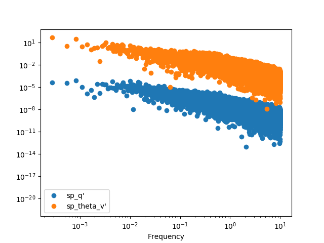
We can plot it with the raw points, but it’s hard to see anything
In [26]: spectra.plot(loglog=True, style='o')
Out[26]: <matplotlib.axes._subplots.AxesSubplot at 0x7f17b321e2d0>

In [27]: plt.show()
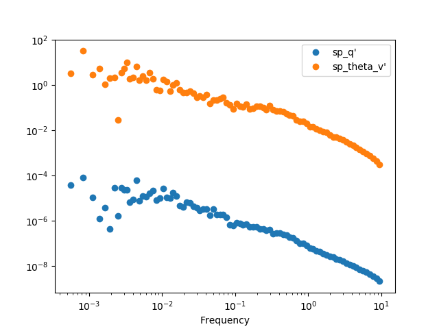
The best option it to apply a binning procedure before plotting it:
In [28]: spectra.binned(bins_number=100).plot(loglog=True, style='o')
Out[28]: <matplotlib.axes._subplots.AxesSubplot at 0x7f17c6ad66d0>

In [29]: plt.show()
We can also calculate the cross-spectra
In [30]: crspectra = pm.crossSpectra(ddata[["q'", "theta_v'", "w'"]], frequency=20, anti_aliasing=True)

In [31]: print(crspectra)
                                              X_q'_theta_v'  \
Frequency
0.000000                        (1.2782144802581139e-17+0j)
0.000278       (0.04314040748364735-0.0065685770458882775j)
0.000556       (0.009094189816514926+0.006795548469370172j)
0.000833        (0.04960683561479265+0.008174148251922277j)
0.001111       (0.004841036679377178+0.002581393740468466j)
0.001389   (-0.0025206201755370813+0.00035264183655764705j)
0.001667     (0.0005815312833474133-0.0019181389200497955j)
0.001944    (-0.0004888213309434262+0.0007640719426831074j)
0.002222       (0.006878729487709714+0.003444450168920351j)
0.002500   (-3.200381556594415e-05+0.00021101917370328936j)
0.002778       (0.009144846912029119+0.004126399648711848j)
0.003056       (0.002972813476272077-0.010640663192420583j)
0.003333      (0.014986041209229509+0.0032905700734580812j)
0.003611     (0.0033975859423399668+0.0006045152747653853j)
0.003889      (0.004666862308853523+0.0007767974691521668j)
...                                                     ...
9.996111   (-3.009661550568595e-07-2.0996420666822683e-07j)
9.996389    (9.867241149923764e-07-2.7512591637127613e-06j)
9.996667   (-1.2075642026837439e-06+9.418780670190427e-07j)
9.996944   (-1.8520274933089603e-08-6.150320779652202e-07j)
9.997222    (-3.02777230961334e-07+1.8145659721714944e-07j)
9.997500     (1.862611957370144e-07+2.216417597711243e-08j)
9.997778    (8.745344044038217e-08-1.9413261258850666e-07j)
9.998056    (4.800978062324763e-07-1.3473380643308305e-07j)
9.998333      (1.6826866379744005e-07+3.0139374343779e-07j)
9.998611    (-4.964023286306099e-07-3.314292842696242e-07j)
9.998889    (-7.93045707948233e-07+1.0850450826426473e-06j)
9.999167    (2.7001206766918043e-07-6.299257141769517e-08j)
9.999444   (-6.289293846739959e-07+1.2637676210416415e-07j)
9.999722    (3.3706273459745717e-07-2.347229370639366e-08j)
10.000000                         (7.27769321146335e-07+0j)

                                                     X_q'_w'  \
Frequency
0.000000                         (2.0826284663761992e-19+0j)
0.000278        (-0.00601155363033843+0.007643467880230253j)
0.000556        (0.006620151353730031-0.012703217979467928j)
0.000833      (-0.0006917155567577926+0.007552430496344348j)
0.001111      (-0.002261514810301724+0.0029581511794479222j)
0.001389        (0.0023739922346592474+0.00053661674067619j)
0.001667       (0.0014749048276315024+0.001525818316364917j)
0.001944     (0.00013622195249582514+6.774568837525674e-05j)
0.002222      (0.0029147626914783065-0.0014756689219013245j)
0.002500      (0.0009595229300538983-0.0008658678226785306j)
0.002778      (0.0013065563404253547-0.0017056170670691313j)
0.003056        (0.002206244878639321+0.005674448587471432j)
0.003333     (-0.0025951816530255523-0.0007252882404365827j)
0.003611     (-0.0008278491429983441+0.0029735572807467023j)
0.003889      (-0.0028276226160111333-0.002224525287978884j)
...                                                      ...
9.996111    (-7.462614667719749e-07+1.3488123393439285e-06j)
9.996389     (-1.4766344607708485e-06-2.71710642119159e-07j)
9.996667   (-1.6072803622243803e-06-1.6193223687136366e-07j)
9.996944     (1.289078888063388e-06+2.7937426311028184e-07j)
9.997222     (-4.1184432807352234e-07-4.47580424767448e-08j)
9.997500      (1.172484817020258e-06-7.017849549793708e-08j)
9.997778    (3.5863008199979397e-07-1.0352089168516933e-06j)
9.998056      (5.527367551255886e-07-3.980181638160392e-07j)
9.998333     (-1.865570684539805e-07+9.819275539590345e-08j)
9.998611     (-6.410170071101929e-07-4.066938018499427e-07j)
9.998889      (5.200716044040084e-07+7.169547630251225e-07j)
9.999167   (-1.2874391561153541e-06-4.1744944109453704e-07j)
9.999444   (-2.2133509459493517e-06+1.0251959322894811e-06j)
9.999722   (-4.1992969413910357e-08+1.6535529987102903e-07j)
10.000000                        (3.5203366367745024e-07+0j)

                                              X_theta_v'_w'
Frequency
0.000000                          (4.59920579284689e-15+0j)
0.000278            (-7.468475569963227+7.003001330383288j)
0.000556           (-0.6758078744471754-4.152918331162926j)
0.000833           (0.3435975181630314+4.7654337290559985j)
0.001111          (-0.30849342960452925+1.877678598464479j)
0.001389           (-4.667604243182588-1.7638547254054096j)
0.001667          (-0.5394621147629767+0.9689805425775375j)
0.001944        (-0.03507218673516947-0.32456429753997856j)
0.002222           (0.5318484539226603-0.7174637262769471j)
0.002500        (-0.13477035273379284-0.11035995558739843j)
0.002778          (0.17464918484502587-0.7465496955147631j)
0.003056          (-2.2704874181402617+1.7019851300701352j)
0.003333          (-1.799994987281136-0.10158455661236966j)
0.003611         (-0.15853450127632224+1.6559481273463088j)
0.003889          (-1.5836988303910724-0.8685715023741194j)
...                                                     ...
9.996111   (-5.4022956917920024e-05-0.0005186641957356917j)
9.996389   (-6.122213375118587e-05-0.00037370115807525085j)
9.996667    (0.00044654723213703913+0.0004268293228136195j)
9.996944   (-0.00010361842284996888+0.0004170458358315186j)
9.997222    (0.0003757038372726522+0.00028452374982165216j)
9.997500      (0.0006527253698203526-0.000117577125967661j)
9.997778     (0.0007466016427205429-6.719727920068582e-05j)
9.998056    (0.0010909938490307968-0.00039883670252715626j)
9.998333   (-7.667096230635029e-06+0.00031039078153151335j)
9.998611    (0.0005904833556143353-1.3775638970284115e-05j)
9.998889     (9.29734178260978e-05-0.00028818381507486916j)
9.999167   (-0.00033715146873629365-0.0002033598018724622j)
9.999444   (0.00045149635700841693-0.00010832207879303636j)
9.999722   (-7.980508313748062e-05+0.00024225973280338827j)
10.000000                        (0.0005514964285100905+0j)

[36001 rows x 3 columns]
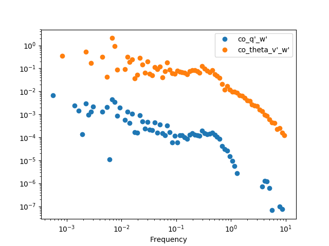
We can then get the cospectra and plot it’s binned version (the same can be
done with the .quadrature() method). It’s important to note that, although
to pass from cross-spectra to cospectra one can merely do
data.apply(np.real), it’s recommended to use the .cospectra() method or
the pm.spectral.cospectra() function, since this way the notation on the
resulting DataFrame will be correctly passed on, as you can see by the legend
in the resulting plot.
In [32]: cospectra = crspectra[[r"X_q'_w'", r"X_theta_v'_w'"]].cospectrum()

In [33]: cospectra.binned(bins_number=100).plot(loglog=True, style='o')
Out[33]: <matplotlib.axes._subplots.AxesSubplot at 0x7f17b3433b10>

In [34]: plt.show()
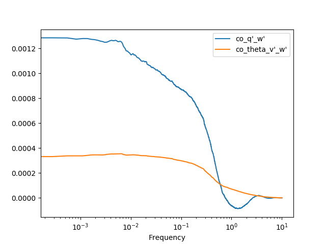
Now we can finally obtain an Ogive with the pm.spectral.Ogive() function.
Note that we plot Og/Og.sum() (i.e. we normalize the ogive) instead of
Og merely for visualization purposes, as the scale of both ogives are too
different.
In [35]: Og = pm.spectral.Ogive(cospectra)

In [36]: (Og/Og.sum()).plot(logx=True)
Out[36]: <matplotlib.axes._subplots.AxesSubplot at 0x7f17b38e6590>

In [37]: plt.show()
Note
Include some examples for spectral corrections.