
Getting started
This “Getting started” tutorial is a brief introduction to Pymicra. This is in no way supposed to be a complete representation of everything that can be done with Pymicra.
In this tutorial we use some example data and refer to some example python scripts that can be downloaded here. These data and scripts are from a measurement campaign in a very small island (about 20 meters across) in a large artificial lake. At the time of these measurements the island was almost completely immersed into about 5 cm of water. Please feel free to explore both the example data and the example programs, as well as modify the programs for your own learning process!
Notation
Pymicra uses a specific notation to name each one of its columns. This notation is extremely important, because it is by these labels that Pymicra knows which variable is in each column. You can check the default notation with
In [1]: %%capture
   ...: import pymicra as pm
   ...: print(pm.notation)
   ...:
The output is too long to be reproduced here, but on the left you’ll see the full name of the variables (which corresponds to a notation namespace/attribute) and on the right you’ll see the default notation for that variable.
We recommend to use the default notation for the sake of simplicity, however,
you can change Pymicra’s notation at any time by altering the attributes of
pm.notation. For example, by default the notation for the mean is
'%s_mean', and every variable follows this base notation:
In [2]: pm.notation.mean
Out[2]: '%s_mean'

In [3]: pm.notation.mean_u
Out[3]: 'u_mean'

In [4]: pm.notation.mean_h2o_mass_concentration
Out[4]: 'conc_h2o_mean'
To change this, you have to change the mean notation and then re-build the
whole notation with the build method:
In [5]: pm.notation.mean = 'm_%s'

In [6]: pm.notation.build()

In [7]: pm.notation.mean_u
Out[7]: 'm_u'

In [8]: pm.notation.mean_h2o_mass_concentration
Out[8]: 'm_conc_h2o'

In [9]: pm.notation.h2o='v'

In [10]: pm.notation.build()

In [11]: pm.notation.mean_h2o_mass_concentration
Out[11]: 'm_conc_v'
If you just want to change the notation of one variable, but not the full notation, just don’t re-build. For example:
In [12]: pm.notation.mean_co2_mass_concentration = 'c_m'

In [13]: pm.notation.mean_co2_mass_concentration
Out[13]: 'c_m'

In [14]: pm.notation.mean_h2o_mass_concentration
Out[14]: 'm_conc_v'
It is important to note that this changes the notation used throughout every Pymicra function. If, however, you want to use a different notation in a specific part of the program (in one specific function for example) you can create a Notation object and pass it to the function, such as
In [15]: mynotation = pm.Notation()

In [16]: mynotation.co2='c'

In [17]: mynotation.build()

In [18]: fluxes = pm.eddyCovariance(data, units, notation=mynotation) # For example
In the example above the default Pymicra notation is left untouched, and a separate notation is defined which is then used in a Pymicra function separately.
Creating file configurations file
The easiest way to read data files is using a fileConfig object. This object holds
the configuration of the data files so you can just call this object when reading these files.
To make it easier, Pymicra prefers to read this configurations from a file. That way
you can write the configurations for some data files once, store it into a configuration file
and then use it from then on every time you want to read those data files. That is what
Pymicra calls a “file configuration file”, or “config file” for short. From that
file, Pymicra can create a pymicra.fileConfig object. Consider, for example, the config
file below
description='datalogger configuration file for a lake. Located at examples/lake.config'

variables={
0:'%Y-%m-%d',
1:'%H:%M:%S.%f',
2:'u',
3:'v',
4:'w',
5:'theta_v',
6:'mrho_h2o',
7:'mrho_co2',
8:'p',
9:'theta'}

units={
'u':'m/s',
'v':'m/s',
'w':'m/s',
'theta_v':'celsius',
'mrho_co2':'mmol/m**3',
'mrho_h2o':'mmol/m**3',
'p':'kPa',
'theta':'celsius'
}

columns_separator=','
frequency=20
header_lines=None

filename_format='%Y%m%d-%H%M.csv'
date_cols = [0, 1]
First of all, note that the .config file is written in Python syntax, so it
has to be able to actually be run on python. This has to be true for all
.config files.
Furthermore, the extension of the file does not matter. We adopt the
.config extension for clarity, but it could be anything else.
The previous config file describes the data files in the directory
../examples/ex_data/. Here’s an example of one such file for comparison:
2013-11-08,10:00:00.000000,2.375,-5.206,-0.103,27.06,1238.0,14.675,99.19,30.43,-0.303,-0.274,-0.269,-0.261
2013-11-08,10:00:00.050000,2.4930000000000003,-5.098,-0.018000000000000002,27.12,1196.0,14.409,99.199,30.43,-0.308,-0.275,-0.271,-0.263
2013-11-08,10:00:00.100000,2.263,-5.114,0.014,27.11,1220.0,14.636,99.102,30.43,-0.306,-0.277,-0.273,-0.263
2013-11-08,10:00:00.150000,2.21,-5.235,-0.012,27.11,1238.0,14.688,99.154,30.43,-0.308,-0.277,-0.273,-0.264
2013-11-08,10:00:00.200000,2.158,-5.174,-0.112,27.12,1174.0,14.476,99.154,30.44,-0.31,-0.277,-0.273,-0.264
2013-11-08,10:00:00.250000,2.334,-5.279,-0.092,27.1,1195.0,14.671,99.154,30.43,-0.308,-0.278,-0.273,-0.265
2013-11-08,10:00:00.300000,2.396,-5.2970000000000015,0.005,27.15,1198.0,14.669,99.154,30.43,-0.309,-0.279,-0.272,-0.264
2013-11-08,10:00:00.350000,2.494,-5.246,0.039,27.13,1197.0,14.722,99.154,30.44,-0.311,-0.279,-0.273,-0.264
2013-11-08,10:00:00.400000,2.263,-5.317,-0.079,27.12,1202.0,14.709,99.154,30.43,-0.311,-0.279,-0.275,-0.265
2013-11-08,10:00:00.450000,2.135,-5.176,-0.036000000000000004,27.08,1202.0,14.731,99.154,30.44,-0.314,-0.279,-0.275,-0.267
Note that not all columns of this file are described. Columns that are not
described are also read but are discarded by default. You can change that using
only_named_columns=False in the timeSeries function.
We obtain the config object with
In [19]: fconfig = pm.fileConfig('../examples/lake.config')

In [20]: print(fconfig)
<pymicra.fileConfig>
datalogger configuration file for a lake. Located at examples/lake.config
Each variable defined in this file works as a keyword, since it can also be
input manually when calling pymicra.fileConfig(). Thus, for more
information, you can also use help(pymicra.fileConfig). Now we explain the
keywords one by one. In the next section we will explain how to use this object
for reading a data file.
description
The description is optional. It’s a string that serves only to better identify the config file you’re dealing with. It might useful for storage purposes and useful when printing the config object.
variables
The most important keyword is variables. This is a python dictionary where
each key is a column and its corresponding value is the variable in that
column. Note that we are using here the default notation to indicate which
variable is in which column. If a different notation is to be used here, then
you will have to define a new notation in your program (refer back to
Notation for that).
Note
From this point on, for simplicity, we will assume that the default notation is used.
It is imperative that the columns be named accordingly. For example, measuring
H2O contents in mmol/m^3 is different from measuring it in g/m^3 or mg/g. The
first is a molar density (moles per volume), the second is a mass density (mass
per volume) and the third is a mass concentration (mass per mass). In the
default notation these are indicated by the names 'mrho_h2o', 'rho_h2o'
and 'conc_h2o', respectively, and Pymicra needs to know which one is which.
Columns that contain parts of the timestamp have to have their name matching Python’s date format string directive, which themselves are the 1989 version default C standard format dates, which is common in many platforms.
This is useful only in case you want to index your data by timestamp, which is a huge advantage in some cases (check out what Pandas can do with timestamp-indexed data) but Pymicra can also work well without this. If you don’t wish to work with timestamps and want to work only by line number in each file, you can ignore these columns and indicate that you don’t want to parse dates. In fact, parsing of dates makes Pymicra a lot slower. Reading a file parsing its dates is about 5.5 times slower than reading the same file without parsing any dates!
units
The units keyword is also very important. It tells Pymicra in which units
each variable is being measured. Units are handled by Pint, so for more
details on how to define the units please refer to their documentation. Suffices
to say here that the format of the units are pretty intuitive. Some quick remarks
are
- prefer to define units unambiguously (
'g/(m*(s**2))'is generally preferred to'g/m/s**2', although both will work).- to define that a unit is dimensionless,
'1'will not work. Define it as'dimensionless'or'g/g'and so on.- if one variable does not have a unit (such as a sensor flag), you don’t have to include that variable.
- the keys of
unitsshould exactly match the values ofvariables.
columns_separator
The columns_separator keyword is what it sounds: what separates one column
from the other. Generally it is one character, such as a comma. A special case
happens is if the columns are separated by whitespaces of varying length, or
tabs. In that case it should be "whitespace".
frequency
The frequency keyword is the frequency of the data collection in Hertz.
header_lines
The keyword header_lines tells us which of the first lines are part of
the file header. If there is no header then is should be None. If there
are header lines than it should be a list or int. For example, if the first two
lines of the file are part of a header, it should be [0, 1]. If it were the
4 first lines, [0, 1, 2, 3] (range(4) would also be acceptable).
Header lines are not used by Pymicra and are therefore skipped.
filename_format
The filename_format keyword tells Pymicra how the data files are named.
date_cols
The date_cols keyword is optional. It is a list of integers that indicates
which of the columns are a part of the timestamp. If it’s not provided, then
Pymicra will assume that columns whose names have the character “%” in them are
part of the date and will try to parse them. If the default notation is used,
this should always be true.
Reading data
To read a data file or a list of data files we use the function timeSeries along with
a config file. Let us use the config file defined in the previous subsection with one of the data
file it describes:
In [21]: fname = '../examples/ex_data/20131108-1000.csv'

In [22]: fconfig = pm.fileConfig('../examples/lake.config')

In [23]: data, units = pm.timeSeries(fname, fconfig, parse_dates=True)

In [24]: print(data)
                             u      v      w  theta_v  mrho_h2o  mrho_co2       p  theta
Timestamp
2013-11-08 10:00:00.000  2.375 -5.206 -0.103    27.06    1238.0    14.675  99.190  30.43
2013-11-08 10:00:00.050  2.493 -5.098 -0.018    27.12    1196.0    14.409  99.199  30.43
2013-11-08 10:00:00.100  2.263 -5.114  0.014    27.11    1220.0    14.636  99.102  30.43
2013-11-08 10:00:00.150  2.210 -5.235 -0.012    27.11    1238.0    14.688  99.154  30.43
2013-11-08 10:00:00.200  2.158 -5.174 -0.112    27.12    1174.0    14.476  99.154  30.44
2013-11-08 10:00:00.250  2.334 -5.279 -0.092    27.10    1195.0    14.671  99.154  30.43
2013-11-08 10:00:00.300  2.396 -5.297  0.005    27.15    1198.0    14.669  99.154  30.43
2013-11-08 10:00:00.350  2.494 -5.246  0.039    27.13    1197.0    14.722  99.154  30.44
2013-11-08 10:00:00.400  2.263 -5.317 -0.079    27.12    1202.0    14.709  99.154  30.43
2013-11-08 10:00:00.450  2.135 -5.176 -0.036    27.08    1202.0    14.731  99.154  30.44
...                        ...    ...    ...      ...       ...       ...     ...    ...
2013-11-08 10:59:59.500  4.951 -4.584  0.420    28.03    1261.0    14.772  99.102  32.08
2013-11-08 10:59:59.550  5.057 -4.436  0.492    28.00    1181.0    14.718  99.138  32.07
2013-11-08 10:59:59.600  5.145 -4.424  0.409    28.10    1216.0    14.889  99.112  32.08
2013-11-08 10:59:59.650  5.282 -4.038  0.448    28.03    1198.0    14.485  99.112  32.06
2013-11-08 10:59:59.700  5.065 -4.453  0.424    28.11    1184.0    14.578  99.138  32.07
2013-11-08 10:59:59.750  5.262 -4.703  0.126    27.98    1264.0    14.929  99.138  32.08
2013-11-08 10:59:59.800  5.323 -4.882  0.242    27.95    1229.0    14.258  99.138  32.07
2013-11-08 10:59:59.850  5.344 -5.119  0.457    27.96    1198.0    14.962  99.102  32.07
2013-11-08 10:59:59.900  5.281 -5.261  0.599    28.09    1231.0    14.615  99.112  32.07
2013-11-08 10:59:59.950  5.235 -4.801  0.362    28.02    1211.0    14.682  99.164  32.08

[72000 rows x 8 columns]
Note that data is a pandas.DataFrame object which contains the whole
data available in the datafile with each column being a variable. Since we
indicated that we wanted to parse the dates with the option
parse_dates=True, each row has its respective timestamp. If, otherwise, we
were to ignore the dates, the result would be a integer-indexed dataset:
In [25]: data2, units = pm.timeSeries(fname, fconfig, parse_dates=False)

In [26]: print(data2)
           u      v      w  theta_v  mrho_h2o  mrho_co2       p  theta
0      2.375 -5.206 -0.103    27.06    1238.0    14.675  99.190  30.43
1      2.493 -5.098 -0.018    27.12    1196.0    14.409  99.199  30.43
2      2.263 -5.114  0.014    27.11    1220.0    14.636  99.102  30.43
3      2.210 -5.235 -0.012    27.11    1238.0    14.688  99.154  30.43
4      2.158 -5.174 -0.112    27.12    1174.0    14.476  99.154  30.44
5      2.334 -5.279 -0.092    27.10    1195.0    14.671  99.154  30.43
6      2.396 -5.297  0.005    27.15    1198.0    14.669  99.154  30.43
7      2.494 -5.246  0.039    27.13    1197.0    14.722  99.154  30.44
8      2.263 -5.317 -0.079    27.12    1202.0    14.709  99.154  30.43
9      2.135 -5.176 -0.036    27.08    1202.0    14.731  99.154  30.44
...      ...    ...    ...      ...       ...       ...     ...    ...
71990  4.951 -4.584  0.420    28.03    1261.0    14.772  99.102  32.08
71991  5.057 -4.436  0.492    28.00    1181.0    14.718  99.138  32.07
71992  5.145 -4.424  0.409    28.10    1216.0    14.889  99.112  32.08
71993  5.282 -4.038  0.448    28.03    1198.0    14.485  99.112  32.06
71994  5.065 -4.453  0.424    28.11    1184.0    14.578  99.138  32.07
71995  5.262 -4.703  0.126    27.98    1264.0    14.929  99.138  32.08
71996  5.323 -4.882  0.242    27.95    1229.0    14.258  99.138  32.07
71997  5.344 -5.119  0.457    27.96    1198.0    14.962  99.102  32.07
71998  5.281 -5.261  0.599    28.09    1231.0    14.615  99.112  32.07
71999  5.235 -4.801  0.362    28.02    1211.0    14.682  99.164  32.08

[72000 rows x 8 columns]
And, as mentioned, the latter way is a lot faster:
In [27]: %timeit pm.timeSeries(fname, fconfig, parse_dates=False)
   ....: %timeit pm.timeSeries(fname, fconfig, parse_dates=True)
   ....:
1 loop, best of 3: 216 ms per loop
1 loop, best of 3: 933 ms per loop
Viewing and manipulating data
To view and manipulate data, mostly you have to follow Pandas’s DataFrame rules. For that we suggest that the user visit a Pandas tutorial. However, I’ll explain some main ideas here for the sake of completeness and introduce some few ideas specific for Pymicra that don’t exist for general Pandas DataFrames.
Printing and plotting
First, for viewing raw data on screen there’s printing. Slicing and indexing are supported by Pandas, but without support for units:
In [29]: print(data['theta_v'])
Timestamp
2013-11-08 10:00:00.000    27.06
2013-11-08 10:00:00.050    27.12
2013-11-08 10:00:00.100    27.11
2013-11-08 10:00:00.150    27.11
2013-11-08 10:00:00.200    27.12
2013-11-08 10:00:00.250    27.10
                           ...
2013-11-08 10:59:59.700    28.11
2013-11-08 10:59:59.750    27.98
2013-11-08 10:59:59.800    27.95
2013-11-08 10:59:59.850    27.96
2013-11-08 10:59:59.900    28.09
2013-11-08 10:59:59.950    28.02
Name: theta_v, Length: 72000, dtype: float64

In [30]: print(data[['u', 'v', 'w']])
                             u      v      w
Timestamp
2013-11-08 10:00:00.000  2.375 -5.206 -0.103
2013-11-08 10:00:00.050  2.493 -5.098 -0.018
2013-11-08 10:00:00.100  2.263 -5.114  0.014
2013-11-08 10:00:00.150  2.210 -5.235 -0.012
2013-11-08 10:00:00.200  2.158 -5.174 -0.112
2013-11-08 10:00:00.250  2.334 -5.279 -0.092
...                        ...    ...    ...
2013-11-08 10:59:59.700  5.065 -4.453  0.424
2013-11-08 10:59:59.750  5.262 -4.703  0.126
2013-11-08 10:59:59.800  5.323 -4.882  0.242
2013-11-08 10:59:59.850  5.344 -5.119  0.457
2013-11-08 10:59:59.900  5.281 -5.261  0.599
2013-11-08 10:59:59.950  5.235 -4.801  0.362

[72000 rows x 3 columns]

In [31]: print(data['20131108 10:15:00.000':'20131108 10:17:00.000'])
                             u      v      w  theta_v  mrho_h2o  mrho_co2       p  theta
Timestamp
2013-11-08 10:15:00.000  2.634 -4.351  0.107    27.30    1229.0    15.002  99.128  30.80
2013-11-08 10:15:00.050  2.869 -4.249  0.040    27.44    1175.0    14.751  99.164  30.80
2013-11-08 10:15:00.100  3.320 -4.326 -0.079    27.26    1159.0    14.689  99.138  30.80
2013-11-08 10:15:00.150  2.759 -4.339 -0.007    27.24    1170.0    14.715  99.190  30.80
2013-11-08 10:15:00.200  2.748 -4.128 -0.038    27.21    1174.0    14.681  99.190  30.80
2013-11-08 10:15:00.250  3.149 -4.074 -0.387    27.20    1190.0    14.662  99.173  30.80
...                        ...    ...    ...      ...       ...       ...     ...    ...
2013-11-08 10:17:00.700  3.910 -4.698 -0.366    27.27    1170.0    14.592  99.128  30.85
2013-11-08 10:17:00.750  3.824 -4.535 -0.313    27.33    1165.0    14.492  99.164  30.85
2013-11-08 10:17:00.800  3.758 -4.353 -0.116    27.28    1103.0    14.495  99.164  30.85
2013-11-08 10:17:00.850  3.761 -4.454 -0.010    27.28    1128.0    14.611  99.164  30.85
2013-11-08 10:17:00.900  3.546 -4.766 -0.433    27.28    1131.0    14.709  99.147  30.85
2013-11-08 10:17:00.950  3.238 -4.601 -0.378    27.29    1130.0    14.809  99.147  30.85

[2420 rows x 8 columns]
Note that Pandas “guesses” if the argument you pass ('theta_v' or
'2013-11-08 10:15:00' etc.) is a column indexer or a row indexer. To use
these unambiguously, use the .loc method as
In [32]: print(data.loc['2013-11-08 10:15:00':'2013-11-08 10:17:00', ['u','v','w']])
                             u      v      w
Timestamp
2013-11-08 10:15:00.000  2.634 -4.351  0.107
2013-11-08 10:15:00.050  2.869 -4.249  0.040
2013-11-08 10:15:00.100  3.320 -4.326 -0.079
2013-11-08 10:15:00.150  2.759 -4.339 -0.007
2013-11-08 10:15:00.200  2.748 -4.128 -0.038
2013-11-08 10:15:00.250  3.149 -4.074 -0.387
...                        ...    ...    ...
2013-11-08 10:17:00.700  3.910 -4.698 -0.366
2013-11-08 10:17:00.750  3.824 -4.535 -0.313
2013-11-08 10:17:00.800  3.758 -4.353 -0.116
2013-11-08 10:17:00.850  3.761 -4.454 -0.010
2013-11-08 10:17:00.900  3.546 -4.766 -0.433
2013-11-08 10:17:00.950  3.238 -4.601 -0.378

[2420 rows x 3 columns]
This method is actually preferred and you can find more information on this topic here.
To view these data with units, you can use the .with_units() method.
The previous output would look like this using units:
In [33]: print(data.with_units(units)['theta_v'])
                         <degC>
Timestamp
2013-11-08 10:00:00.000   27.06
2013-11-08 10:00:00.050   27.12
2013-11-08 10:00:00.100   27.11
2013-11-08 10:00:00.150   27.11
2013-11-08 10:00:00.200   27.12
2013-11-08 10:00:00.250   27.10
...                         ...
2013-11-08 10:59:59.700   28.11
2013-11-08 10:59:59.750   27.98
2013-11-08 10:59:59.800   27.95
2013-11-08 10:59:59.850   27.96
2013-11-08 10:59:59.900   28.09
2013-11-08 10:59:59.950   28.02

[72000 rows x 1 columns]

In [34]: print(data.with_units(units)[['u', 'v', 'w']])
                                       u                v                w
                        <meter / second> <meter / second> <meter / second>
Timestamp
2013-11-08 10:00:00.000            2.375           -5.206           -0.103
2013-11-08 10:00:00.050            2.493           -5.098           -0.018
2013-11-08 10:00:00.100            2.263           -5.114            0.014
2013-11-08 10:00:00.150            2.210           -5.235           -0.012
2013-11-08 10:00:00.200            2.158           -5.174           -0.112
2013-11-08 10:00:00.250            2.334           -5.279           -0.092
...                                  ...              ...              ...
2013-11-08 10:59:59.700            5.065           -4.453            0.424
2013-11-08 10:59:59.750            5.262           -4.703            0.126
2013-11-08 10:59:59.800            5.323           -4.882            0.242
2013-11-08 10:59:59.850            5.344           -5.119            0.457
2013-11-08 10:59:59.900            5.281           -5.261            0.599
2013-11-08 10:59:59.950            5.235           -4.801            0.362

[72000 rows x 3 columns]

In [35]: print(data.with_units(units)['2013-11-08 10:15:00'])
                                       u                v                w theta_v  \
                        <meter / second> <meter / second> <meter / second>  <degC>
Timestamp
2013-11-08 10:15:00.000            2.634           -4.351            0.107   27.30
2013-11-08 10:15:00.050            2.869           -4.249            0.040   27.44
2013-11-08 10:15:00.100            3.320           -4.326           -0.079   27.26
2013-11-08 10:15:00.150            2.759           -4.339           -0.007   27.24
2013-11-08 10:15:00.200            2.748           -4.128           -0.038   27.21
2013-11-08 10:15:00.250            3.149           -4.074           -0.387   27.20
...                                  ...              ...              ...     ...
2013-11-08 10:15:00.700            3.057           -4.090           -0.230   27.28
2013-11-08 10:15:00.750            3.386           -4.169           -0.082   27.21
2013-11-08 10:15:00.800            3.731           -4.180            0.291   27.42
2013-11-08 10:15:00.850            3.676           -4.100            0.021   27.29
2013-11-08 10:15:00.900            3.796           -4.390            0.170   27.24
2013-11-08 10:15:00.950            3.294           -3.322            0.560   27.50

                                        mrho_h2o                 mrho_co2            p  theta
                        <millimole / meter ** 3> <millimole / meter ** 3> <kilopascal> <degC>
Timestamp
2013-11-08 10:15:00.000                   1229.0                   15.002       99.128   30.8
2013-11-08 10:15:00.050                   1175.0                   14.751       99.164   30.8
2013-11-08 10:15:00.100                   1159.0                   14.689       99.138   30.8
2013-11-08 10:15:00.150                   1170.0                   14.715       99.190   30.8
2013-11-08 10:15:00.200                   1174.0                   14.681       99.190   30.8
2013-11-08 10:15:00.250                   1190.0                   14.662       99.173   30.8
...                                          ...                      ...          ...    ...
2013-11-08 10:15:00.700                   1151.0                   14.758       99.164   30.8
2013-11-08 10:15:00.750                   1195.0                   14.318       99.164   30.8
2013-11-08 10:15:00.800                   1172.0                   14.369       99.164   30.8
2013-11-08 10:15:00.850                   1173.0                   14.687       99.164   30.8
2013-11-08 10:15:00.900                   1153.0                   14.442       99.164   30.8
2013-11-08 10:15:00.950                   1176.0                   14.724       99.208   30.8

[20 rows x 8 columns]
Warning
Note that, although this method returns a Pandas DataFrame, it is not meant for calculations. Currently the DataFrame it returns is meant for visualization purposes only!
We can also plot the data on screen so we can view it interactively. This can be done directly from the DataFrame with
In [36]: from matplotlib import pyplot as plt

In [37]: data[['u', 'v', 'w']].plot()
Out[37]: <matplotlib.axes._subplots.AxesSubplot at 0x7f17c7956950>

In [38]: plt.show()
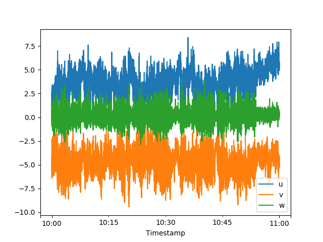
Using the plt.show() command, the plot above would plot interactively. If
we had used plt.savefig('figure.png') instead, it would have saved the
figure as png. For more on plotting, you can checkout Pandas’s visualization
guide and
find out ways to make this plot look nicer, how to render it with LaTeX and
some more tricks.
Pymicra also has an .xplot method, which brings a little more options to
Pandas’s .plot() method.
Todo
give xplot examples
Converting units
You can manually convert between units using the contents from Manipulating
and the Pint package. But Pymicra has a very useful method to do this called .convert_cols (more exist,
but let’s focus on this one).
Let’s, for example, convert some units:
In [39]: conversions = {'p':'pascal', 'mrho_h2o':'mole/m^3', 'theta_v':'kelvin'}

In [40]: print(data.convert_cols(conversions, units, inplace_units=False))
(                             u      v      w  theta_v  mrho_h2o  mrho_co2        p  theta
Timestamp
2013-11-08 10:00:00.000  2.375 -5.206 -0.103   300.21     1.238    14.675  99190.0  30.43
2013-11-08 10:00:00.050  2.493 -5.098 -0.018   300.27     1.196    14.409  99199.0  30.43
2013-11-08 10:00:00.100  2.263 -5.114  0.014   300.26     1.220    14.636  99102.0  30.43
2013-11-08 10:00:00.150  2.210 -5.235 -0.012   300.26     1.238    14.688  99154.0  30.43
2013-11-08 10:00:00.200  2.158 -5.174 -0.112   300.27     1.174    14.476  99154.0  30.44
2013-11-08 10:00:00.250  2.334 -5.279 -0.092   300.25     1.195    14.671  99154.0  30.43
...                        ...    ...    ...      ...       ...       ...      ...    ...
2013-11-08 10:59:59.700  5.065 -4.453  0.424   301.26     1.184    14.578  99138.0  32.07
2013-11-08 10:59:59.750  5.262 -4.703  0.126   301.13     1.264    14.929  99138.0  32.08
2013-11-08 10:59:59.800  5.323 -4.882  0.242   301.10     1.229    14.258  99138.0  32.07
2013-11-08 10:59:59.850  5.344 -5.119  0.457   301.11     1.198    14.962  99102.0  32.07
2013-11-08 10:59:59.900  5.281 -5.261  0.599   301.24     1.231    14.615  99112.0  32.07
2013-11-08 10:59:59.950  5.235 -4.801  0.362   301.17     1.211    14.682  99164.0  32.08

[72000 rows x 8 columns], {'theta_v': <Unit('kelvin')>, 'p': <Unit('pascal')>, 'mrho_h2o': <Unit('mole / meter ** 3')>})
Note that the units dictionary is updated automatically if the
inplace_units keyword is true. The default is false for safety reasons, but
passing this keyword as true is much simpler and compact:
In [41]: conversions = {'theta':'kelvin', 'theta_v':'kelvin'}

In [42]: data = data.convert_cols(conversions, units, inplace_units=True)

In [43]: print(data.with_units(units))
                                       u                v                w  theta_v  \
                        <meter / second> <meter / second> <meter / second> <kelvin>
Timestamp
2013-11-08 10:00:00.000            2.375           -5.206           -0.103   300.21
2013-11-08 10:00:00.050            2.493           -5.098           -0.018   300.27
2013-11-08 10:00:00.100            2.263           -5.114            0.014   300.26
2013-11-08 10:00:00.150            2.210           -5.235           -0.012   300.26
2013-11-08 10:00:00.200            2.158           -5.174           -0.112   300.27
2013-11-08 10:00:00.250            2.334           -5.279           -0.092   300.25
...                                  ...              ...              ...      ...
2013-11-08 10:59:59.700            5.065           -4.453            0.424   301.26
2013-11-08 10:59:59.750            5.262           -4.703            0.126   301.13
2013-11-08 10:59:59.800            5.323           -4.882            0.242   301.10
2013-11-08 10:59:59.850            5.344           -5.119            0.457   301.11
2013-11-08 10:59:59.900            5.281           -5.261            0.599   301.24
2013-11-08 10:59:59.950            5.235           -4.801            0.362   301.17

                                        mrho_h2o                 mrho_co2            p    theta
                        <millimole / meter ** 3> <millimole / meter ** 3> <kilopascal> <kelvin>
Timestamp
2013-11-08 10:00:00.000                   1238.0                   14.675       99.190   303.58
2013-11-08 10:00:00.050                   1196.0                   14.409       99.199   303.58
2013-11-08 10:00:00.100                   1220.0                   14.636       99.102   303.58
2013-11-08 10:00:00.150                   1238.0                   14.688       99.154   303.58
2013-11-08 10:00:00.200                   1174.0                   14.476       99.154   303.59
2013-11-08 10:00:00.250                   1195.0                   14.671       99.154   303.58
...                                          ...                      ...          ...      ...
2013-11-08 10:59:59.700                   1184.0                   14.578       99.138   305.22
2013-11-08 10:59:59.750                   1264.0                   14.929       99.138   305.23
2013-11-08 10:59:59.800                   1229.0                   14.258       99.138   305.22
2013-11-08 10:59:59.850                   1198.0                   14.962       99.102   305.22
2013-11-08 10:59:59.900                   1231.0                   14.615       99.112   305.22
2013-11-08 10:59:59.950                   1211.0                   14.682       99.164   305.23

[72000 rows x 8 columns]
Manipulating
Manipulating data is pretty intuitive with Pandas. For example
In [44]: data['rho_air'] = data['p']/(287.058*data['theta_v'])

In [45]: print(data['rho_air'])
Timestamp
2013-11-08 10:00:00.000    0.001151
2013-11-08 10:00:00.050    0.001151
2013-11-08 10:00:00.100    0.001150
2013-11-08 10:00:00.150    0.001150
2013-11-08 10:00:00.200    0.001150
2013-11-08 10:00:00.250    0.001150
                             ...
2013-11-08 10:59:59.700    0.001146
2013-11-08 10:59:59.750    0.001147
2013-11-08 10:59:59.800    0.001147
2013-11-08 10:59:59.850    0.001147
2013-11-08 10:59:59.900    0.001146
2013-11-08 10:59:59.950    0.001147
Name: rho_air, Length: 72000, dtype: float64
If, however, you’re not familiar with Pandas and prefer to just stick with what
you know, you can get Numpy arrays from columns using the .values
attribute:
In [46]: P = data['p'].values

In [47]: Tv = data['theta_v'].values

In [48]: print(type(Tv))
<type 'numpy.ndarray'>

In [49]: rho_air = P/(287.058*Tv)

In [50]: print(rho_air)
[0.00115099 0.00115087 0.00114978 ... 0.00114654 0.00114616 0.00114702]

In [51]: print(type(rho_air))
<type 'numpy.ndarray'>
Doing that you can step out of Pandas and do your own calculations using your own Python or Numpy code. This is pretty advantageous if you have a lot of routines that are already written in your own way.