
Hands-on tutorial
Here we give some examples of generally-used steps to obtain fluxes, spectra and Ogives. This is just the commonly done procedures, but more can (and sometimes should) be done depending on the data.
Calculating auxiliary variables and units
After reading the data it’s easy to rotate the coordinates. Currently, only the
2D rotation is implemented. But in the future more will come (you can
contribute with another one yourself!). To rotate, use the pm.rotateCoor
function:
In [1]: import pymicra as pm

In [2]: fname = '../examples/ex_data/20131108-1000.csv'

In [3]: fconfig = pm.fileConfig('../examples/lake.config')

In [4]: data, units = pm.timeSeries(fname, fconfig, parse_dates=True)

In [5]: data = data.rotateCoor(how='2d')

In [6]: print(data.with_units(units).mean())
u         <meter / second>            6.021737e+00
v         <meter / second>            2.271683e-14
w         <meter / second>            1.178001e-16
theta_v   <degC>                      2.764434e+01
mrho_h2o  <millimole / meter ** 3>    1.169865e+03
mrho_co2  <millimole / meter ** 3>    1.466232e+01
p         <kilopascal>                9.913677e+01
theta     <degC>                      3.127128e+01
dtype: float64
As you can see, the u, v, w components have been rotated and v and w
mean are zero.
Pymicra has a very useful function called preProcess which “expands” the
variables in the dataset by using the original variables to calculate new ones,
such as mixing ratios, moist and dry air densities etc. In the process some
units are also converted, such as temperature units, which are converted to
Kelvin, if they are in Celsius. The preProcess function has some options to
calculate some variables in determined ways and is very “verbose”, so as to
show the user exactly what it is doing:
In [7]: data = pm.preProcess(data, units, expand_temperature=True,
   ...:     use_means=False, rho_air_from_theta_v=True, solutes=['co2'])
   ...:
Beginning of pre-processing ...
Converting theta_v and theta to kelvin ... Done!
Didn't locate mass density of h2o. Trying to calculate it ... Done!
Moist air density not present in dataset
Calculating rho_air = p/(Rdry * theta_v) ... Done!
Calculating dry_air mass_density = rho_air - rho_h2o ... Done!
Dry air molar density not in dataset
Calculating dry_air molar_density = rho_dry / dry_air_molar_mass ... Done!
Calculating specific humidity = rho_h2o / rho_air ... Done!
Calculating h2o mass mixing ratio = rho_h2o / rho_dry ... Done!
Calculating h2o molar mixing ratio = rho_h2o / rho_dry ... Done!
Didn't locate mass density of co2. Trying to calculate it ... Done!
Calculating co2 mass concentration (g/g) = rho_co2 / rho_air ... Done!
Calculating co2 mass mixing ratio = rho_co2 / rho_dry ... Done!
Calculating co2 molar mixing ratio = mrho_co2 / mrho_dry ... Done!
Pre-processing complete.


In [8]: print(data.with_units(units).mean())
u         <meter / second>            6.021737e+00
v         <meter / second>            2.271683e-14
w         <meter / second>            1.178001e-16
theta_v   <kelvin>                    3.007943e+02
mrho_h2o  <millimole / meter ** 3>    1.169865e+03
mrho_co2  <millimole / meter ** 3>    1.466232e+01
p         <kilopascal>                9.913677e+01
theta     <kelvin>                    3.044213e+02
rho_h2o   <kilogram / meter ** 3>     2.107547e-02
rho_air   <kilogram / meter ** 3>     1.148149e+00
rho_dry   <kilogram / meter ** 3>     1.127073e+00
mrho_dry  <mole / meter ** 3>         3.891223e+01
q         <dimensionless>             1.835686e-02
r_h2o     <dimensionless>             1.870102e-02
mr_h2o    <dimensionless>             3.006698e-02
rho_co2   <kilogram / meter ** 3>     6.452812e-04
conc_co2  <dimensionless>             5.620179e-04
r_co2     <dimensionless>             5.725280e-04
mr_co2    <dimensionless>             3.768047e-04
dtype: float64
Note that our dataset now has many other variables and that the temperatures are now in Kelvin. Note also that you must, at this point, specify which solutes you wish to consider. The only solute that Pymicra looks for by default is water vapor.
It is recommended that you carefully observe the output of preProcess to
see if it’s doing what you think it’s doing and to analyse its calculation
logic. By doing that you can have a better idea of what it does without having
to check the code, and how to prevent it from doing some calculations you don’t
want. For example, if you’re not happy with the way it calculates moist air
density, you can calculate it yourself by extracting Numpy_ arrays using the
.values method:
T = data['theta'].values
P = data['p'].values
water_density = data['mrho_h2o'].values
data['rho_air'] = my_rho_air_calculation(T, P, water_density)
Next we calculate the fluctuations. The way to do that is with the detrend()
function/method.
In [9]: ddata = data.detrend(how='linear', units=units, ignore=['p', 'theta'])

In [10]: print(ddata.with_units(units).mean())
u'         <meter / second>            1.071294e-08
v'         <meter / second>            1.889055e-08
w'         <meter / second>            8.740592e-10
theta_v'   <kelvin>                    6.261396e-09
mrho_h2o'  <millimole / meter ** 3>    1.206199e-07
mrho_co2'  <millimole / meter ** 3>   -5.600283e-10
rho_h2o'   <kilogram / meter ** 3>     7.408674e-13
rho_air'   <kilogram / meter ** 3>     3.606646e-12
rho_dry'   <kilogram / meter ** 3>     9.526920e-12
mrho_dry'  <mole / meter ** 3>        -2.731307e-09
q'         <dimensionless>             2.835312e-13
r_h2o'     <dimensionless>             2.301367e-12
mr_h2o'    <dimensionless>             1.006615e-11
rho_co2'   <kilogram / meter ** 3>     2.048293e-14
conc_co2'  <dimensionless>            -1.126744e-14
r_co2'     <dimensionless>            -4.827255e-15
mr_co2'    <dimensionless>            -1.057082e-14
dtype: float64
Note the ignore keyword with which you can pass which variables you don’t
want fluctuations of. In our case both the pressure fluctuations and the
thermodynamic temperature (measured with the LI7500 and the datalogger’s
internal thermometer) can’t be properly measured with the sensors used. Passing
these variables as ignored will prevent Pymicra from calculating these
fluctuations, which later on prevents it from inadvertently using the
fluctuations of these variables with these sensors when calculating fluxes.
theta fluctuations will instead be calculated with virtual temperature
fluctuations and pressure fluctuations are generally not used.
The how keyword supports 'linear', 'movingmean',
'movingmedian', 'block' and 'poly'. Each of those (with the
exception of 'block' and 'linear') are passed to Pandas or Numpy
(pandas.rolling_mean, pandas.rolling_median and numpy.polyfit) and
support their respective keywords, such as data.detrend(how='movingmedian',
units=units, ignore=['theta', 'p']), min_periods=1) to determine the minimum
number of observations in window required to have a value.
Now we must expand our dataset with the fluctuations by joining DataFrames:
In [11]: data = data.join(ddata)

In [12]: print(data.with_units(units).mean())
u          <meter / second>            6.021737e+00
v          <meter / second>            2.271683e-14
w          <meter / second>            1.178001e-16
theta_v    <kelvin>                    3.007943e+02
mrho_h2o   <millimole / meter ** 3>    1.169865e+03
mrho_co2   <millimole / meter ** 3>    1.466232e+01
p          <kilopascal>                9.913677e+01
theta      <kelvin>                    3.044213e+02
rho_h2o    <kilogram / meter ** 3>     2.107547e-02
rho_air    <kilogram / meter ** 3>     1.148149e+00
rho_dry    <kilogram / meter ** 3>     1.127073e+00
mrho_dry   <mole / meter ** 3>         3.891223e+01
q          <dimensionless>             1.835686e-02
r_h2o      <dimensionless>             1.870102e-02
mr_h2o     <dimensionless>             3.006698e-02
                                           ...
w'         <meter / second>            8.740592e-10
theta_v'   <kelvin>                    6.261396e-09
mrho_h2o'  <millimole / meter ** 3>    1.206199e-07
mrho_co2'  <millimole / meter ** 3>   -5.600283e-10
rho_h2o'   <kilogram / meter ** 3>     7.408674e-13
rho_air'   <kilogram / meter ** 3>     3.606646e-12
rho_dry'   <kilogram / meter ** 3>     9.526920e-12
mrho_dry'  <mole / meter ** 3>        -2.731307e-09
q'         <dimensionless>             2.835312e-13
r_h2o'     <dimensionless>             2.301367e-12
mr_h2o'    <dimensionless>             1.006615e-11
rho_co2'   <kilogram / meter ** 3>     2.048293e-14
conc_co2'  <dimensionless>            -1.126744e-14
r_co2'     <dimensionless>            -4.827255e-15
mr_co2'    <dimensionless>            -1.057082e-14
Length: 36, dtype: float64
Creating a site configuration file
In order to use some micrometeorological function, we need a site configuration
object, or site object. This object tells Pymicra how the instruments are organized
and how is experimental site (vegetation, roughness length etc.). This object is created
with the siteConfig() call and the easiest way is to use it with a site config file. This
is like a fileConfig file, but simpler and for the micrometeorological aspects of the site.
Consider this example of a site config file, saved at ../examples/lake.site:
description         = "Site configurations for the lake island"

measurement_height  = 2.75  # m
canopy_height       = 0.1   # m
displacement_height = 0.05  # m
roughness_length    = .01   # m
As in the case of fileConfig, the description is optional, but is handy for
organization purposes and printing on screen.
The measurement_height keyword is the general measurement height to be used
in the calculation, generally taken as the sonic anemometer height (in meters).
The canopy_height keyword is what it sounds like. Should be the mean canopy
height in meters. The displacement_height is the zero-plane displacement
height. If it is not given, it’ll be calculated as 2/3 of the mean canopy
height.
The roughness_length is the roughness length in meters.
The creation of the site config object is done as
In [13]: siteconf = pm.siteConfig('../examples/lake.site')

In [14]: print(siteconf)
<pymicra.siteConfig> object
Site configurations for the lake island
----
altitude               None
canopy_height           0.1
displacement_height    0.05
from_file              None
instruments_height     None
latitude               None
longitude              None
measurement_height     2.75
roughness_length       0.01
dtype: object
Extracting fluxes
Finally, we are able to calculate the fluxes and turbulent scales. For that we
use the eddyCovariance function along with the get_turbulent_scales
keyword (which is true by default). Again, it is recommended that you carefully
check the output of this function before moving on:
In [15]: results = pm.eddyCovariance(data, units, site_config=siteconf,
   ....:     get_turbulent_scales=True, wpl=True, solutes=['co2'])
   ....:
Beginning Eddy Covariance method...
Fluctuations of theta not found. Will try to calculate it with theta' = (theta_v' - 0.61 theta_mean q')/(1 + 0.61 q_mean ... done!
Calculating fluxes from covariances ... done!
Applying WPL correction for water vapor flux ... done!
Applying WPL correction for latent heat flux using result for water vapor flux ... done!
Re-calculating cov(mrho_h2o', w') according to WPL correction ... done!
Applying WPL correction for F_co2 ... done!
Re-calculating cov(mrho_co2', w') according to WPL correction ... done!
Beginning to extract turbulent scales...
Data seems to be covariances. Will it use as covariances ...
Calculating the turbulent scales of wind, temperature and humidity ... done!
Calculating the turbulent scale of co2 ... done!
Calculating Obukhov length and stability parameter ... done!
Calculating turbulent scales of mass concentration ... done!
Done with Eddy Covariance.


In [16]: print(results.with_units(units).mean())
tau            <kilogram / meter / second ** 2>     1.957307e-01
H              <watt / meter ** 2>                  5.083720e+01
Hv             <watt / meter ** 2>                  7.453761e+01
E              <millimole / meter ** 2 / second>    7.007486e+00
LE             <watt / meter ** 2>                  3.063926e+02
F_co2          <millimole / meter ** 2 / second>    2.648931e-04
u_star         <meter / second>                     4.128863e-01
theta_v_star   <kelvin>                             1.566857e-01
theta_star     <kelvin>                             1.068650e-01
mrho_h2o_star  <millimole / meter ** 3>             1.697195e+01
mrho_co2_star  <millimole / meter ** 3>             6.415643e-04
Lo             <meter>                             -8.342964e+01
zeta           <dimensionless>                     -3.236260e-02
q_star         <dimensionless>                      2.663024e-04
conc_co2_star  <dimensionless>                      2.459169e-08
dtype: float64
Note that once more we must list the solutes available.
Note also that the units dictionary is automatically updated at with every
function and method with the new variables created and their units! That way if
you’re in doubt of which unit the outputs are coming, just check units
directly or with the .with_units() method.
Check out the example to get fluxes of many files here and download the example data here.
The output of this file is
                                                 tau                   H                  Hv                                 E                  LE  \
                    <kilogram / meter / second ** 2> <watt / meter ** 2> <watt / meter ** 2> <millimole / meter ** 2 / second> <watt / meter ** 2>
2013-11-08 10:00:00                         0.195731           50.837195           74.537609                          7.007486          306.392623
2013-11-08 12:00:00                         0.070182           -7.116972           14.737946                          6.647450          290.331014
2013-11-08 13:00:00                         0.059115           -3.325774           12.743194                          4.875838          212.906974
2013-11-08 16:00:00                         0.017075          -13.847040           -4.131275                          2.961474          128.982980
2013-11-08 17:00:00                         0.003284           -5.557620           -2.525949                          0.931213           40.576805
2013-11-08 18:00:00                         0.026564           -6.632330           -2.782190                          1.184226           51.654208
2013-11-08 19:00:00                         0.044550          -14.860873          -11.991508                          0.925637           40.476446

                              u_star theta_v_star theta_star            mrho_h2o_star          Lo            zeta          q_star
                    <meter / second>     <kelvin>   <kelvin> <millimole / meter ** 3>     <meter> <dimensionless> <dimensionless>
2013-11-08 10:00:00         0.412886     0.156686   0.106865                16.971952  -83.429641       -0.032363        0.000266
2013-11-08 12:00:00         0.247697     0.051834  -0.025031                26.837060  -90.992476       -0.029673        0.000423
2013-11-08 13:00:00         0.227652     0.048903  -0.012763                21.417958  -81.621514       -0.033080        0.000338
2013-11-08 16:00:00         0.122980    -0.029651  -0.099383                24.080946   39.583979        0.068209        0.000384
2013-11-08 17:00:00         0.053951    -0.041353  -0.090986                17.260443    5.463569        0.494182        0.000276
2013-11-08 18:00:00         0.153328    -0.016003  -0.038149                 7.723494  113.854892        0.023714        0.000123
2013-11-08 19:00:00         0.198083    -0.053132  -0.065846                 4.672974   56.961515        0.047400        0.000074
Note that the date parsing when reading the file comes is handy now, although
there are computationally faster ways to do it other than setting
parse_dates=True in the timeSeries() call.
Obtaining the spectra
Using Numpy’s fast Fourier transform implementation, Pymicra is also able to extract spectra, co-spectra and quadratures.
We begin normally with out data:
In [17]: import pymicra as pm

In [18]: fname = '../examples/ex_data/20131108-1000.csv'

In [19]: fconfig = pm.fileConfig('../examples/lake.config')

In [20]: data, units = pm.timeSeries(fname, fconfig, parse_dates=True)

In [21]: data = data.rotateCoor(how='2d')

In [22]: data = pm.preProcess(data, units, expand_temperature=True,
   ....:     use_means=False, rho_air_from_theta_v=True, solutes=['co2'])
   ....:
Beginning of pre-processing ...
Converting theta_v and theta to kelvin ... Done!
Didn't locate mass density of h2o. Trying to calculate it ... Done!
Moist air density not present in dataset
Calculating rho_air = p/(Rdry * theta_v) ... Done!
Calculating dry_air mass_density = rho_air - rho_h2o ... Done!
Dry air molar density not in dataset
Calculating dry_air molar_density = rho_dry / dry_air_molar_mass ... Done!
Calculating specific humidity = rho_h2o / rho_air ... Done!
Calculating h2o mass mixing ratio = rho_h2o / rho_dry ... Done!
Calculating h2o molar mixing ratio = rho_h2o / rho_dry ... Done!
Didn't locate mass density of co2. Trying to calculate it ... Done!
Calculating co2 mass concentration (g/g) = rho_co2 / rho_air ... Done!
Calculating co2 mass mixing ratio = rho_co2 / rho_dry ... Done!
Calculating co2 molar mixing ratio = mrho_co2 / mrho_dry ... Done!
Pre-processing complete.


In [23]: ddata = data.detrend(how='linear', units=units, ignore=['p', 'theta'])

In [24]: spectra = pm.spectra(ddata[["q'", "theta_v'"]], frequency=20, anti_aliasing=True)

In [25]: print(spectra)
                  sp_q'   sp_theta_v'
Frequency
0.000000   5.788056e-22  2.822765e-13
0.000278   4.144722e-05  4.594375e+01
0.000556   3.865066e-05  3.334581e+00
0.000833   7.980519e-05  3.167281e+01
0.001111   1.073580e-05  2.803632e+00
0.001389   1.241472e-06  5.217905e+00
0.001667   3.835354e-06  1.047474e+00
0.001944   4.227172e-07  1.946342e+00
0.002222   2.814147e-05  2.102988e+00
0.002500   1.583606e-06  2.876558e-02
0.002778   2.811465e-05  3.580177e+00
0.003056   2.370466e-05  5.149254e+00
0.003333   2.293235e-05  1.026538e+01
0.003611   6.403198e-06  1.859856e+00
0.003889   9.423592e-06  2.375211e+00
...                 ...           ...
9.996111   1.084777e-09  1.241413e-04
9.996389   1.158869e-08  7.371886e-04
9.996667   4.004893e-09  5.856201e-04
9.996944   1.888643e-09  2.004653e-04
9.997222   3.102855e-10  4.015675e-04
9.997500   3.321963e-10  1.059147e-04
9.997778   3.111850e-10  1.456869e-04
9.998056   2.923886e-10  8.503993e-04
9.998333   2.343816e-10  5.083698e-04
9.998611   7.671555e-10  4.643917e-04
9.998889   3.931099e-09  4.594757e-04
9.999167   9.530669e-10  8.066022e-05
9.999444   3.370132e-09  1.221089e-04
9.999722   2.259948e-10  5.051543e-04
10.000000  4.645530e-10  1.140124e-03

[36001 rows x 2 columns]
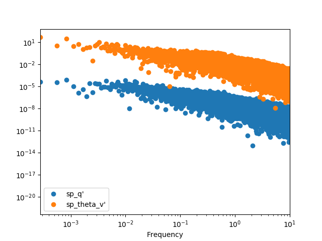
We can plot it with the raw points, but it’s hard to see anything
In [26]: spectra.plot(loglog=True, style='o')
Out[26]: <matplotlib.axes._subplots.AxesSubplot at 0x7f0f4c65ad50>

In [27]: plt.show()
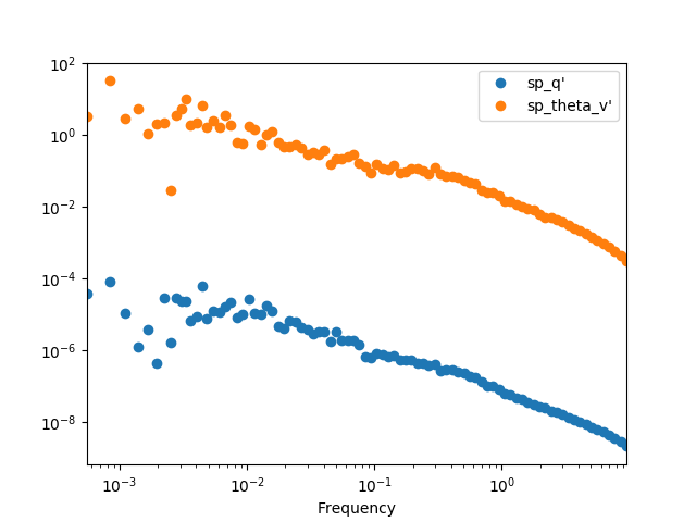
The best option it to apply a binning procedure before plotting it:
In [28]: spectra.binned(bins_number=100).plot(loglog=True, style='o')
Out[28]: <matplotlib.axes._subplots.AxesSubplot at 0x7f0f4d302e90>

In [29]: plt.show()
We can also calculate the cross-spectra
In [30]: crspectra = pm.crossSpectra(ddata[["q'", "theta_v'", "w'"]], frequency=20, anti_aliasing=True)

In [31]: print(crspectra)
                                     X_q'_theta_v'                                  X_q'_w'  \
Frequency
0.000000                    (1.27821448026e-17+0j)                   (1.78432291667e-18+0j)
0.000278       (0.0431404074836-0.00656857704589j)    (-0.00601155363032+0.00764346788022j)
0.000556      (0.00909418981651+0.00679554846937j)      (0.00662015135376-0.0127032179794j)
0.000833       (0.0496068356148+0.00817414825192j)   (-0.000691715556873+0.00755243049633j)
0.001111      (0.00484103667938+0.00258139374047j)    (-0.00226151481031+0.00295815117946j)
0.001389    (-0.00252062017554+0.000352641836558j)    (0.00237399223466+0.000536616740677j)
0.001667     (0.000581531283347-0.00191813892005j)     (0.00147490482763+0.00152581831637j)
0.001944   (-0.000488821330943+0.000764071942683j)   (0.000136221952496+6.77456883715e-05j)
0.002222      (0.00687872948771+0.00344445016892j)     (0.00291476269146-0.00147566892192j)
0.002500   (-3.20038155659e-05+0.000211019173703j)   (0.000959522930054-0.000865867822675j)
0.002778      (0.00914484691203+0.00412639964871j)     (0.00130655634042-0.00170561706705j)
0.003056       (0.00297281347627-0.0106406631924j)     (0.00220624487865+0.00567444858753j)
0.003333       (0.0149860412092+0.00329057007346j)   (-0.00259518165305-0.000725288240451j)
0.003611     (0.00339758594234+0.000604515274765j)   (-0.000827849142993+0.00297355728073j)
0.003889     (0.00466686230885+0.000776797469152j)      (-0.002827622616-0.00222452528797j)
...                                            ...                                      ...
9.996111   (-3.00966155057e-07-2.09964206668e-07j)  (-7.46261466835e-07+1.34881233931e-06j)
9.996389    (9.86724114992e-07-2.75125916371e-06j)  (-1.47663446102e-06-2.71710642356e-07j)
9.996667   (-1.20756420268e-06+9.41878067019e-07j)  (-1.60728036222e-06-1.61932236836e-07j)
9.996944   (-1.85202749331e-08-6.15032077965e-07j)    (1.2890788879e-06+2.79374263104e-07j)
9.997222   (-3.02777230961e-07+1.81456597217e-07j)    (-4.1184432809e-07-4.4758042452e-08j)
9.997500    (1.86261195737e-07+2.21641759771e-08j)   (1.17248481701e-06-7.01784954967e-08j)
9.997778    (8.74534404404e-08-1.94132612589e-07j)    (3.5863008201e-07-1.03520891683e-06j)
9.998056    (4.80097806232e-07-1.34733806433e-07j)   (5.52736755132e-07-3.98018163818e-07j)
9.998333    (1.68268663797e-07+3.01393743438e-07j)    (-1.86557068434e-07+9.819275541e-08j)
9.998611    (-4.96402328631e-07-3.3142928427e-07j)  (-6.41017007125e-07-4.06693801792e-07j)
9.998889   (-7.93045707948e-07+1.08504508264e-06j)   (5.20071604376e-07+7.16954762957e-07j)
9.999167    (2.70012067669e-07-6.29925714177e-08j)  (-1.28743915612e-06-4.17449441124e-07j)
9.999444   (-6.28929384674e-07+1.26376762104e-07j)   (-2.21335094617e-06+1.0251959323e-06j)
9.999722    (3.37062734597e-07-2.34722937064e-08j)   (-4.19929694132e-08+1.6535529989e-07j)
10.000000                   (7.27769321146e-07+0j)                   (3.52033663677e-07+0j)

                                     X_theta_v'_w'
Frequency
0.000000                      (3.940437974e-14+0j)
0.000278           (-7.46847556994+7.00300133038j)
0.000556          (-0.675807874437-4.15291833116j)
0.000833           (0.343597518091+4.76543372906j)
0.001111          (-0.308493429603+1.87767859847j)
0.001389           (-4.66760424319-1.76385472541j)
0.001667         (-0.539462114765+0.968980542578j)
0.001944        (-0.0350721867423-0.324564297536j)
0.002222           (0.531848453917-0.71746372628j)
0.002500         (-0.134770352733-0.110359955587j)
0.002778          (0.174649184847-0.746549695508j)
0.003056           (-2.27048741817+1.70198513008j)
0.003333           (-1.7999949873-0.101584556618j)
0.003611          (-0.158534501275+1.65594812734j)
0.003889          (-1.58369883039-0.868571502373j)
...                                            ...
9.996111   (-5.40229568945e-05-0.000518664195739j)
9.996389   (-6.12221337163e-05-0.000373701158155j)
9.996667    (0.000446547232145+0.000426829322803j)
9.996944   (-0.000103618422846+0.000417045835778j)
9.997222    (0.000375703837303+0.000284523749807j)
9.997500    (0.000652725369815-0.000117577125966j)
9.997778     (0.000746601642711-6.7197279189e-05j)
9.998056     (0.00109099384904-0.000398836702528j)
9.998333   (-7.66709619807e-06+0.000310390781516j)
9.998611    (0.000590483355599-1.37756390144e-05j)
9.998889     (9.2973417813e-05-0.000288183815053j)
9.999167   (-0.000337151468736-0.000203359801881j)
9.999444     (0.00045149635705-0.000108322078788j)
9.999722   (-7.98050831385e-05+0.000242259732832j)
10.000000                    (0.00055149642851+0j)

[36001 rows x 3 columns]
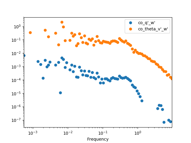
We can then get the cospectra and plot it’s binned version (the same can be
done with the .quadrature() method). It’s important to note that, although
to pass from cross-spectra to cospectra one can merely do
data.apply(np.real), it’s recommended to use the .cospectra() method or
the pm.spectral.cospectra() function, since this way the notation on the
resulting DataFrame will be correctly passed on, as you can see by the legend
in the resulting plot.
In [32]: cospectra = crspectra[[r"X_q'_w'", r"X_theta_v'_w'"]].cospectrum()

In [33]: cospectra.binned(bins_number=100).plot(loglog=True, style='o')
Out[33]: <matplotlib.axes._subplots.AxesSubplot at 0x7f0f4d13fdd0>

In [34]: plt.show()
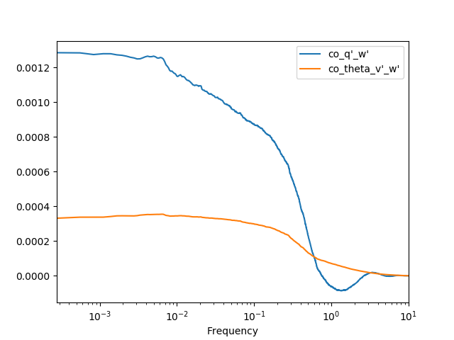
Now we can finally obtain an Ogive with the pm.spectral.Ogive() function.
Note that we plot Og/Og.sum() (i.e. we normalize the ogive) instead of
Og merely for visualization purposes, as the scale of both ogives are too
different.
In [35]: Og = pm.spectral.Ogive(cospectra)

In [36]: (Og/Og.sum()).plot(logx=True)
Out[36]: <matplotlib.axes._subplots.AxesSubplot at 0x7f0f4d02d3d0>

In [37]: plt.show()
Note
Include some examples for spectral corrections.